How to Add Up Columns in Microsoft Excel: 6 Easy Methods

If Excel had a love language, it would be adding things up. And if you’ve ever stared at a column of numbers thinking, “Surely there’s a button for this,” congratulations: Excel has several buttons for this. Some are fast. Some are fancy. One is basically Excel whispering the answer to you from the bottom of the screen like a helpful ghost.

In this guide, you’ll learn six easy, real-world ways to add up columns in Microsoft Excelplus how to avoid the classic “Why is my total wrong?” heartbreak. We’ll go from one-click totals to smarter formulas that handle filters, hidden rows, and criteria.

Before You Sum: What “Add Up a Column” Really Means

“Add up a column” sounds simple until Excel gets picky (or you do). Before you choose a method, decide what you’re actually trying to total:

• Everything in the column? Even future rows you’ll add later?
• Only a specific range? Like this month’s data (B2:B31), not last year’s mystery numbers below.
• Only visible rows? Because you filtered the list and don’t want hidden rows included.
• Only certain items? Like “East” region sales, or orders over $500.

Excel can handle all of that. The trick is picking the right tool so you don’t end up summing your header, your subtotal, and your dignity.

Method 1: AutoSum (The One-Click “Do It For Me” Button)

AutoSum is the easiest way to total a column when your numbers are in a clean block. It automatically inserts a SUM formula and guesses the range. Most of the time, it guesses correctlylike a well-trained golden retriever.

How to use AutoSum

1. Click the cell directly below the last number in your column (for example, click B12 if data is in B2:B11).
2. Go to Home (or Formulas) > AutoSum (∑).
3. Press Enter to accept the suggested range.

Keyboard shortcut (Windows)

Select the total cell and press Alt + =. Excel drops in the SUM formula instantly. It’s the closest thing Excel has to a mic drop.

Example

If your values are in C2:C10, AutoSum will likely create:
=SUM(C2:C10)

Pro tip: If Excel highlights the wrong range, don’t panic. Just drag to select the correct cells and press Enter.

Method 2: The SUM Function (Manual Control, Maximum Flexibility)

The SUM function is the foundation of most totals in Excel. It’s simple, reliable, and doesn’t get weird unless you tell it to. You can sum a range, multiple ranges, or even an entire column.

Basic range sum

Click the cell where you want the total, then type:
=SUM(A2:A100)

Sum multiple columns (or separate ranges)

Want to add up two columns at once?
=SUM(B2:B20, D2:D20)

Sum an entire column (use with care)

You can total a whole column like this:
=SUM(D:D)

This is great for quick work, but be cautious in real spreadsheets:

• It includes everything in that columntoday’s data and tomorrow’s accidental paste.
• If you put the total inside the same column you’re summing, you can create a circular reference.
• On massive workbooks, full-column formulas can slow things down.

Fix “numbers stored as text” (the silent total-killer)

If SUM returns 0 or ignores values, some “numbers” may actually be text (often from imports). Quick checks:

• Numbers aligned left by default
• Green triangle warning in the cell
• Status bar shows Count but not Sum

Common fixes:

• Use Convert to Number from the warning icon.
• Use Text to Columns (even without splitting) to coerce text to numbers.
• Multiply by 1 in a helper column: =A2*1
• Use =VALUE(A2) if you need a clean conversion.

Method 3: Excel Table “Total Row” (Dynamic Totals That Grow With Your Data)

If your data changes (and whose doesn’t?), Excel Tables are the grown-up way to sum columns. Turn your range into a table and add a Total Row. Your totals update automatically when you add new rowsno formula babysitting required.

How to add a Total Row

1. Click any cell in your dataset.
2. Create a table: Insert > Table (or press Ctrl + T).
3. Check “My table has headers” if applicable, then click OK.
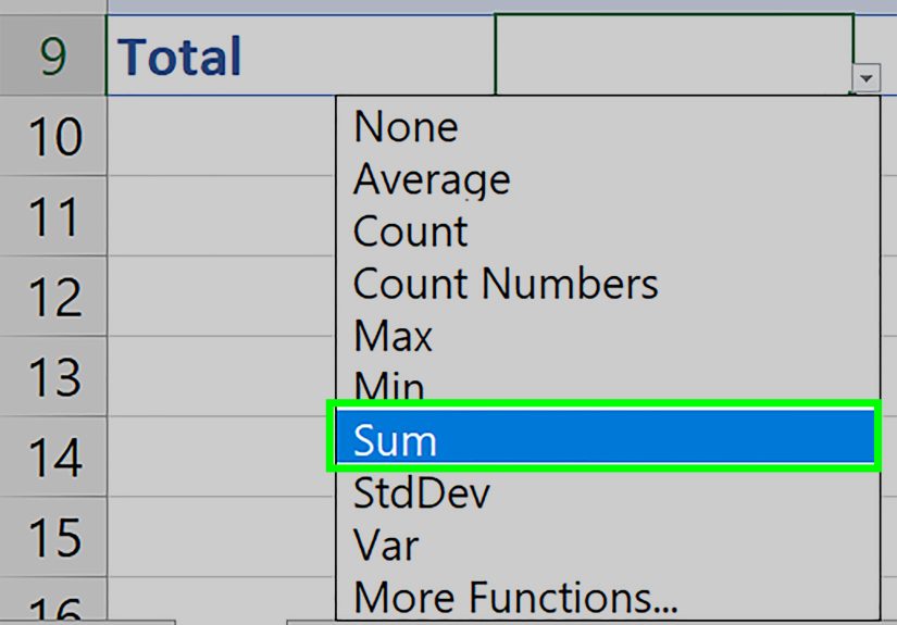
4. Go to Table Design (Table Tools) and check Total Row.
5. In the Total Row under the column you want to add, open the dropdown and choose Sum.

Why this is awesome

• Totals automatically include new rows.
• Formulas use readable structured references (table/column names instead of cryptic ranges).
• Tables play nicely with filters and consistent formatting.

Example idea: A “Sales” column in a table might total with something like:

=SUBTOTAL(109,Table1[Sales])

(Excel often uses SUBTOTAL in table totals so filtered rows behave the way humans expect. Which is rare and beautiful.)

Method 4: The Status Bar Sum (Instant Total Without Any Formula)

Need a quick total but don’t want to change your sheet? Excel can show you the sum of selected cells on the Status Bar at the bottom of the window. This is perfect for quick checks like, “Do these invoices roughly match the payment I received?”

How to use it

1. Select the cells in the column you want to total (for example, drag from B2 to B50).
2. Look at the bottom of Excel for Sum.

If you don’t see “Sum”

1. Right-click the Status Bar.
2. Make sure Sum is checked.

Best for: quick validation and sanity checks.
Not ideal for: totals you need to print, reference, or reuse in other formulas.

Method 5: Quick Analysis Totals (Ctrl + Q for Fast “Add a Total Row/Column”)

Quick Analysis is like Excel’s “suggestion engine” for your selected data. It can add totals with previews, which is handy when you want to total rows/columns without building formulas from scratch.

How to use Quick Analysis

1. Select your data range (including the column you want to total).
2. Click the Quick Analysis icon that appears near the bottom-right of the selection, or press Ctrl + Q.
3. Choose Totals.
4. Select Sum (Excel previews where the total will gohover first if you like living safely).

Why people love it

• Fast totals with visual previews.
• Great for ad-hoc analysis when you don’t want to design a “perfect” spreadsheet.
• Also offers Average, Count, % Total, and Running Total options depending on your selection.

Note: Quick Analysis is available in modern Excel versions (Excel 2013 and later in desktop Excel).

Method 6: Smart Totals for Real Life (SUBTOTAL, SUMIF, and SUMIFS)

Sometimes you don’t want the sum of everything. You want the sum of the right thingslike visible rows after filtering, or sales from one region, or only transactions above a certain amount. This is where “smart totals” earn their keep.

Use SUBTOTAL to sum only visible (filtered) rows

If you filter a list, a normal SUM will still include hidden rows. SUBTOTAL can ignore rows hidden by filters, which makes it perfect for filtered tables.

Common SUBTOTAL formulas for sums:

• =SUBTOTAL(9, B2:B200)  → sums visible rows; ignores rows hidden by a filter
• =SUBTOTAL(109, B2:B200) → also ignores manually hidden rows

When to use it: dashboards, filtered reports, “show me only Q1” lists, and anything where you expect the total to change when you filter.

Use SUMIF to total based on one condition

SUMIF adds values that match a single criterion.

Example: Sum Sales in B2:B100 where Region in A2:A100 equals “East”:
=SUMIF(A2:A100,"East",B2:B100)

Use SUMIFS to total based on multiple conditions

SUMIFS adds values when multiple criteria are met.

Example: Sum Sales in C2:C200 where Region is “East” and Amount is at least 1000:
=SUMIFS(C2:C200, A2:A200, "East", B2:B200, ">=1000")

Why this matters: Filters are great for viewing, but formulas like SUMIF/SUMIFS are better when you need repeatable, auditable totals that update automatically.

Common “Why Is My Total Wrong?” Problems (And Fast Fixes)

1) Your range missed a few cells

AutoSum and manual ranges can accidentally stop early if there are blank rows or stray text cells. Fix it by selecting the range explicitly (for example, change =SUM(B2:B48) to =SUM(B2:B55)).

2) Some values are text

If imported data looks numeric but won’t add, convert text-to-number using the warning icon, Text to Columns, or VALUE.

3) You filtered data but used SUM

If totals don’t change when you filter, switch to SUBTOTAL (or use a Table Total Row).

4) You accidentally included your total cell in the total

This can create a circular reference. Put totals below the data (not inside it), or use a Table Total Row.

5) Hidden rows you forgot about are still included

If someone hid rows manually, use SUBTOTAL(109,...) to ignore those too.

Conclusion: Pick the Total That Matches Your Reality

The best way to add up columns in Excel depends on what you’re doing:

• Fast and simple: AutoSum (or Alt+=)
• Flexible and classic: SUM
• Data that grows: Table Total Row
• Quick sanity check: Status Bar sum
• Instant analysis tools: Quick Analysis
• Filtered/criteria-based totals: SUBTOTAL, SUMIF, SUMIFS

Once you match the method to the situation, Excel stops feeling like a puzzle and starts feeling like… well, a calculator with better outfits.

Experience Notes (Real-World Lessons From Adding Up Columns)

The first time most people “add up a column,” it’s for something innocentlike totaling expenses for a trip or summing quiz scores. Then real life shows up with a spreadsheet that has imports, filters, hidden rows, and at least one column labeled “Final_Final_REALLYFINAL.” That’s usually when Excel totals become less about math and more about trust.

One of the most useful habits I’ve seen in workplaces is using the Status Bar sum as a quick lie detector. Before you even write a formula, you highlight the range and glance at the bottom of Excel. If the sum looks wildly offsay, you expected ~$12,000 and Excel whispers “3”you know you’re dealing with text numbers, blanks, or the wrong selection. That five-second check can save you from building a “perfect” dashboard on top of bad data.

The second big lesson: filters change what humans think “total” means. People will filter to “February” and expect the total to reflect February. If you used SUM, your number doesn’t change, and suddenly you’re in a meeting explaining that the spreadsheet is “technically correct.” (A phrase that never makes anyone happier.) This is why SUBTOTAL becomes a quiet hero in reporting work. If the total should respond to filtering, SUBTOTAL is often the correct choice.

Another common experience: spreadsheets that grow every week. Budgets, inventory logs, timesheetsthese aren’t static. If you hardcode =SUM(B2:B50) and someone adds new rows, your total becomes a time capsule. Converting the range into an Excel Table and turning on the Total Row solves this permanently. The table expands as data expands, and the total stays accurate without anyone remembering to “update the formula.”

And then there’s the “numbers stored as text” problem, which is basically Excel’s version of wearing a fake mustache. Imports from PDFs, copied values from websites, and certain system exports love turning real numbers into text. The sheet looks normal, but SUM ignores the values and your total is wrong. After you’ve been burned once, you start recognizing the signs: left-aligned numbers, weird apostrophes, and totals that refuse to behave. Fixing it (Convert to Number, Text to Columns, VALUE, or multiply by 1) becomes a standard cleanup steplike washing produce before you cook.

Finally, when you move beyond “add everything” and into “add the right things,” SUMIF and SUMIFS become game-changers. In sales reporting, it’s often not useful to total the entire column; you want “East region,” “this quarter,” “only completed orders,” or “projects above a threshold.” Filtering can help you view it, but SUMIFS helps you prove itrepeatably, transparently, and without relying on someone remembering which filter settings were applied.

If there’s a single takeaway from real spreadsheet work, it’s this: Excel totals are easyuntil context matters. The moment context matters (filters, growth, criteria, imports), choosing the correct method is what separates a “total” from a trustworthy number you can present with a straight face.