Table of Contents >> Show >> Hide
- Quick Cheat Sheet (If You’re in a Hurry)
- Why Hide Columns Instead of Deleting Them?
- Step 1: Select the Columns You Want to Hide (Fast)
- Step 2: Right-Click & Hide (The 2-Second Method)
- Step 3: Use the Ribbon (Best for “Where Is That Right-Click Again?” Moments)
- Step 4: Use Keyboard Shortcuts (Speed Mode)
- Step 5: Verify What’s Hidden, Manage It, and Avoid Accidental “Where Did My Data Go?”
- Bonus: How to Unhide Columns (Because You’ll Need This in 3 Minutes)
- Hiding vs. Grouping vs. Filtering (Choose the Right Tool)
- Troubleshooting: Common “Why Won’t Excel Do the Thing?” Issues
- Wrap-Up: Your 5-Step Workflow (One Last Time)
- Experiences & Real-World Scenarios (500+ Words)
Excel is basically a big grid of secrets. Sometimes those secrets are harmless (helper formulas), sometimes they’re sensitive (salary bands), and sometimes they’re just ugly (that one “DO NOT TOUCH” column someone made in 2017 and nobody’s brave enough to delete).
The good news: hiding columns in Excel is fast, tidy, and reversible. The even better news: you don’t need to be an Excel wizardjust someone who knows where the Hide button is hiding (yes, I did that).
Quick Cheat Sheet (If You’re in a Hurry)
- Select the column(s) you want to hide.
- Right-click the column letter(s) → choose Hide.
- Or use the Ribbon: Home → Format → Hide & Unhide → Hide Columns.
- Keyboard shortcut (Windows): Ctrl + 0 (zero).
- Keyboard shortcut (Mac): ⌘ + 0 (zero) in many setups.
Why Hide Columns Instead of Deleting Them?
Hiding is perfect when you want a cleaner view without breaking formulas, references, or layouts. Deleting columns can shift data, wreck formulas, and cause your spreadsheet to develop a personality. Hiding keeps the structure intact while letting you present only what matters.
Common reasons people hide columns:
- Presenting summaries: Show the dashboard, hide the messy plumbing.
- Keeping helper columns out of sight: VLOOKUP/XLOOKUP keys, staging areas, lookup tables.
- Reducing distractions: Less scrolling, fewer “what is this?” questions.
- Temporarily masking sensitive info: (Important note: hiding is not securitymore on that later.)
Step 1: Select the Columns You Want to Hide (Fast)
Most “Excel is hard” moments are actually “selecting is annoying” moments. Here are quick ways to select columns like you mean it.
Option A: Click the Column Letter (The Classic)
Click the letter at the top (A, B, C…) to select the entire column. If you click inside the column’s cells, you might only select a cellExcel will absolutely take that personally.
Option B: Select a Range of Adjacent Columns (Shift)
- Click the first column letter (for example, C).
- Hold Shift, then click the last column letter (for example, G).
- You’ve now selected C:G.
Option C: Select Non-Adjacent Columns (Ctrl/Command)
- Click the first column letter you want (say, B).
- Hold Ctrl (Windows) or ⌘ (Mac).
- Click other columns (for example, E and H).
- Now you can hide multiple “islands” of columns at once.
Option D: Keyboard Selection (When You’re Feeling Efficient)
- Ctrl + Space selects the current column (based on the active cell).
- Then use Shift + Arrow keys to expand selection (depends on your layout).
Option E: The Name Box Trick for Huge Ranges
Need to hide a massive stretch like columns D through CE without dragging until next Tuesday? Click the Name Box (left of the formula bar), type:
Press Enter, and Excel selects the whole column range instantly. This is a lifesaver for financial models, timelines, and any sheet that’s basically “columns forever.”
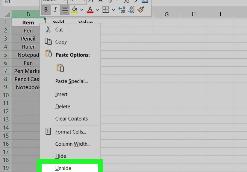
Step 2: Right-Click & Hide (The 2-Second Method)
Once your columns are selected, the fastest method is the context menu:
- Right-click any selected column letter.
- Click Hide.
That’s it. Your columns vanish, leaving a thin double-line indicator between the surrounding columns. Think of it as Excel’s way of saying, “Don’t worry, I didn’t delete anything… probably.”
Example: You have a budget sheet where columns D:F contain raw transaction detail, and columns G:J are summaries. Hide D:F before sharing the file with stakeholders who only need the big picture.
Step 3: Use the Ribbon (Best for “Where Is That Right-Click Again?” Moments)
If you prefer the Ribbonespecially in corporate environments where right-click menus feel like forbidden magicdo this:
- Select the column(s).
- Go to Home.
- In the Cells group, click Format.
- Choose Hide & Unhide → Hide Columns.
Ribbon navigation is also handy when you’re teaching someone else and want a predictable path they can follow. (“Click Home, then Format…” is easier than “Right-click… no not there… no, the letter… okay close enough.”)
Step 4: Use Keyboard Shortcuts (Speed Mode)
If you hide columns frequently, shortcuts save real timeespecially on wide sheets where mouse travel becomes cardio.
Windows Shortcut
- Hide selected columns: Ctrl + 0 (zero)
Mac Shortcut (Often)
- Hide selected columns: ⌘ + 0 (zero) in many Excel-for-Mac setups
If Your Shortcut Doesn’t Work (Because Computers Love Drama)
Sometimes shortcut keys get hijacked by system settings, regional keyboard layouts, or organizational policies. If Ctrl + 0 (or the unhide shortcut you try later) isn’t cooperating, don’t panicuse the Ribbon method (Step 3), or use Excel’s Key Tips sequence for unhiding (shown in the Bonus section below).
Pro Tip: If you want a “shortcut-like” fallback, add Hide Columns to your Quick Access Toolbar. Then you can trigger it with Alt + a number key (Windows), depending on its position. This is great when your keyboard shortcuts are restricted by IT policies.
Step 5: Verify What’s Hidden, Manage It, and Avoid Accidental “Where Did My Data Go?”
Hidden columns are easy to spot once you know the signs:
- A double line appears between column letters where hidden columns exist.
- Column letters jump (you’ll see A, B, E… meaning C and D are hidden).
Make Hidden Columns Harder to Unhide (For Sharing)
If you’re sharing a sheet and want to discourage others from unhiding columns (for example, hiding internal notes or helper logic), you can protect the sheet and restrict formatting actions. This can gray out Hide/Unhide options for recipients. Just remember: protection is a control, not a fortress.
Important: Hiding Is Not Security
Hidden columns can be revealed by anyone who knows how to unhide themso don’t treat hiding like encryption. For truly sensitive information, use proper permissions, file protection, and data governance practices.
Bonus: How to Unhide Columns (Because You’ll Need This in 3 Minutes)
Even if your goal is “hide,” your future self will eventually say, “Okay, now show them again.” Here are the fastest ways to unhide.
Method 1: Select Adjacent Columns → Right-Click → Unhide
- Select the columns immediately before and after the hidden columns.
- Right-click the selection.
- Choose Unhide.
Method 2: Double-Click the Hidden Indicator Line
If you see the double line between, say, columns B and E, double-click that line to unhide what’s in between.
Method 3: The Ribbon Unhide Path
Home → Format → Hide & Unhide → Unhide Columns
Method 4: Keyboard Sequence for Unhide (Works Even When Ctrl+Shift+0 Doesn’t)
On Windows, a reliable way to unhide via the Ribbon Key Tips is:
Alt, then H, then O, then U, then L
(That’s Home → Format → Hide & Unhide → Unhide Columns.)
Special Case: Unhide Column A (The “It’s Gone and I Can’t Select It” Problem)
If column A is hidden, unhiding can feel weird because there’s nothing “to the left” to select. One common approach:
- Select the whole sheet (click the triangle in the top-left corner between row numbers and column letters).
- Go to Home → Format → Hide & Unhide → Unhide Columns.
Hiding vs. Grouping vs. Filtering (Choose the Right Tool)
Excel gives you multiple “clean up the view” options. They look similar, but they behave differently:
| Tool | Best For | What It Does | Watch Out For |
|---|---|---|---|
| Hide Columns | Temporary cleanup, hiding helper columns | Makes columns invisible until unhidden | Not secure; easy to unhide |
| Group (Outline) | Collapsible sections (monthly detail, line-item drilldowns) | Adds +/- toggles to expand/collapse column groups | Requires setup; can confuse first-time viewers |
| Filter | Hiding rows based on criteria | Shows only rows that match selections | Doesn’t hide columns; changes what data is visible |
If you want your users to expand/collapse sections on demand, grouping is often better than hiding. If you just want columns out of the way, hiding is perfect.
Troubleshooting: Common “Why Won’t Excel Do the Thing?” Issues
1) “I can hide columns, but I can’t unhide them with a shortcut.”
This is surprisingly common. If Ctrl + Shift + 0 doesn’t work on Windows, use one of these:
- Right-click adjacent columns → Unhide
- Ribbon path: Home → Format → Hide & Unhide → Unhide Columns
- Key Tips sequence: Alt H O U L
2) “My printed sheet looks wrong after hiding columns.”
Printing depends on page breaks, scaling, and print areas. After hiding columns, quickly check:
- Print Area (Page Layout → Print Area)
- Scaling (File → Print → Scaling options)
- Page Break Preview (View → Page Break Preview)
3) “I hid columns in Excel Online and now something’s inconsistent.”
Excel for the web generally supports hiding columns through the column header menu and context actions, but some view modes (like certain “Sheet View” behaviors) may not preserve hidden states the way you expect. If persistence matters, confirm in the default view and save.
Wrap-Up: Your 5-Step Workflow (One Last Time)
- Select the column(s) (Shift for ranges, Ctrl/⌘ for non-adjacent, Name Box for huge ranges).
- Right-click → Hide (fastest for most people).
- Or go Home → Format → Hide & Unhide → Hide Columns.
- Use shortcuts: Ctrl + 0 (Windows), often ⌘ + 0 (Mac).
- Confirm and manage hidden columns; protect the sheet if you need to discourage unhiding.
Experiences & Real-World Scenarios (500+ Words)
Below are some common “in the wild” situations where hiding columns saves time, prevents confusion, and occasionally stops a spreadsheet from starting a small office fire. (Metaphorically. Mostly.)
Scenario 1: The Executive Dashboard That Needed a Glow-Up
A typical reporting sheet often has two personalities: the polished summary on the left and the chaotic data engine on the right. The summary might show revenue totals, key variances, and a couple of charts. Meanwhile, the “engine” includes lookup tables, helper columns for cleaning text, and intermediate steps that make the final numbers correct but are painful to look at. Hiding columns becomes the difference between “This report is easy to read” and “Why are there 47 columns titled TEMP?” In practice, the cleanest workflow is to hide the helper columns before meetings, then unhide them afterward when you need to troubleshoot. It keeps stakeholders focused on decisionsnot the behind-the-scenes duct tape that makes the sheet work.
Scenario 2: Financial Models and the Endless Timeline
If you’ve ever built a model with monthly periods stretching into the far future, you already know the pain: you only need the next 12–24 months for most discussions, but the spreadsheet insists on showing 10 years of columns. A slick trick is to keep the full timeline available but hide the distant months until needed. When someone asks, “Can we see the impact in year five?” you unhide the relevant range and look like a wizard who anticipated everything. Using the Name Box to select large ranges (like D:CE) makes this practicalotherwise you’ll spend more time selecting columns than analyzing them. The best part: hiding doesn’t break formulas or assumptions; it just reduces visual noise.
Scenario 3: Shared Sheets and the “Please Don’t Touch That” Problem
In shared workbooks, people mean well… and then accidentally type over a helper column that drives every calculation. Hiding columns helps, but it’s not enough on its own because anyone can unhide. The real-world approach is layered: hide the helper columns for cleanliness, then protect the sheet to limit who can unhide or format columns. This works especially well when you’re sharing with clients or cross-functional teams who should edit inputs but not the logic. You’re basically creating a “front stage” and “back stage” experience: inputs and outputs stay visible, while the logic stays tucked away. It’s not perfect security, but it dramatically reduces accidental damage.
Scenario 4: Data Cleaning Without Scaring People
Data cleaning often requires temporary columns: splitting names, extracting IDs, standardizing dates, removing extra spaces, and building new “clean” values next to messy originals. The problem is that when other people open the sheet, they see those extra columns and assume they’re part of the final structure. Hiding “workbench” columns solves this. A common pattern is to keep the raw imported data visible (for transparency), hide the intermediate cleanup columns, and keep the final cleaned output visible. When questions pop up“Where did this value come from?”you can unhide the workbench briefly, explain, and then re-hide so the sheet stays readable. It’s like showing someone the kitchen only when they ask how the meal was made.