
Table of Contents >> Show >> Hide
- Why use multiple lines in one Excel graph?
- Before you start: set up your data the smart way
- Way 1: Create a multiple-line graph from one data table
- Way 2: Add more lines to an existing Excel chart
- Way 3: Use a combo chart or scatter-style setup for tricky data
- What to do if Excel graphs the wrong lines
- Best practices for a clearer multi-line chart
- Example: comparing three product lines
- Common mistakes to avoid
- Experiences people often have when graphing multiple lines in Excel
- Conclusion
- SEO Tags
If Excel charts have ever made you feel like your spreadsheet is judging you, welcome to the club. The good news is that graphing multiple lines in Excel is much easier than it first appears. Once your data is organized properly, Excel can turn a plain worksheet into a clear visual that shows trends, comparisons, and those little “aha” moments that make numbers finally behave.
This guide walks through 3 easy ways to graph multiple lines in Excel, including how to create a multi-line chart from scratch, how to add more lines to an existing graph, and how to handle situations where your data uses different scales or awkward x-axis values. Along the way, you’ll also learn how to fix common chart problems without dramatically whispering, “Why are you like this?” at your monitor.
Why use multiple lines in one Excel graph?
A multiple-line graph is useful when you want to compare trends across two or more data series in the same chart. Instead of flipping between separate visuals, you can see how several sets of values move over time or across categories in one place. That makes it easier to compare sales by product, website traffic by channel, temperatures by city, or monthly expenses by department.
In plain English: one line tells a story, but multiple lines let the stories gossip about each other.
Before you start: set up your data the smart way
Before creating a line graph in Excel, make sure your worksheet is arranged in a clean table format. In most cases, the first column should contain your category labels or dates, and each additional column should represent a separate data series.
| Month | North Region | South Region | West Region |
|---|---|---|---|
| January | 120 | 95 | 110 |
| February | 135 | 100 | 118 |
| March | 140 | 108 | 125 |
| April | 150 | 112 | 132 |
This layout helps Excel recognize that “Month” belongs on the horizontal axis and each region should become its own line. If your data is messy, merged, or scattered like it survived a windstorm, your chart may come out equally confused.
Way 1: Create a multiple-line graph from one data table
This is the fastest and most common method. If all the data series you want to compare are already in one table, Excel can build the chart in just a few clicks.
Step 1: Select the full data range
Click and drag to highlight the entire table, including the labels in the top row and the dates or categories in the first column. Don’t skip the headers. Without them, your legend may end up looking like “Series 1,” “Series 2,” and “Series 3,” which is technically accurate and emotionally unhelpful.
Step 2: Go to the Insert tab
On the Excel ribbon, click Insert. In the Charts group, choose Line or Insert Line or Area Chart. Then pick a standard 2-D Line chart. In many cases, Line with Markers is even better because it makes each data point easier to see.
Step 3: Let Excel build the chart
Once you click the chart type, Excel creates a graph with multiple lines automatically. Each column becomes a separate series, and the first column usually becomes the x-axis.
Step 4: Clean up the chart
A chart that works is nice. A chart people can actually read is better. Add these finishing touches:
- Chart title: Make it specific, such as “Quarterly Sales by Region.”
- Axis titles: Label the horizontal and vertical axes.
- Legend: Keep it visible so readers know which line is which.
- Gridlines: Use lightly for readability, not as decorative prison bars.
- Colors: Choose distinct colors so lines do not blend together.
When this method works best
Use this method when your data is already organized in adjacent columns or rows and all your series share the same type of scale. It is ideal for monthly trends, performance comparisons, or simple year-over-year visuals.
Way 2: Add more lines to an existing Excel chart
Sometimes you already have one line graph in Excel, and then someone says, “Can we add two more departments, last year’s data, and maybe a forecast?” Of course they do. Fortunately, Excel lets you add more lines without starting over.
Step 1: Click the existing chart
Select the chart you already created. This tells Excel you are editing the current visual rather than building a new one from scratch.
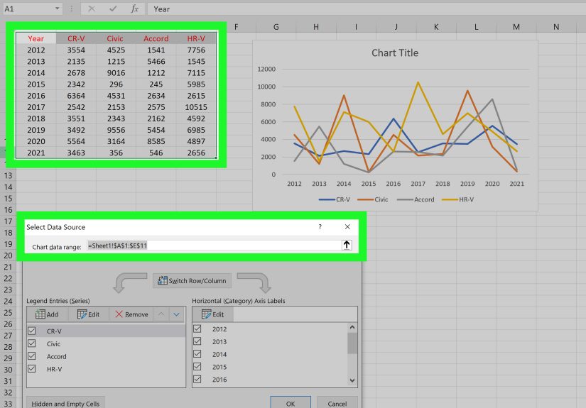
Step 2: Open Select Data
Right-click the chart and choose Select Data. This opens the Select Data Source dialog box, which is where you can add, edit, rearrange, or remove chart series.
Step 3: Add a new series
In the Legend Entries (Series) section, click Add. Then choose:
- Series name: the header cell for the new line
- Series values: the numeric values for that line
If necessary, update the horizontal axis labels as well so the dates or categories match across every series.
Step 4: Repeat for additional lines
You can repeat the process to add as many lines as needed. Just remember that “as many as Excel allows” and “as many as humans can read” are not the same number. In practice, too many lines can make a chart look like spaghetti attending a business meeting.
Step 5: Reorder the series if needed
Inside the same Select Data window, you can move series up or down. This can help with legend order and can sometimes improve which line appears on top when lines overlap.
When this method works best
Use this method when you already have a chart and want to add new data series later. It is especially useful for dashboards, reports that get updated monthly, and charts that evolve as your project grows.
Way 3: Use a combo chart or scatter-style setup for tricky data
Not all data behaves nicely. Sometimes one line represents sales in dollars while another shows conversion rate as a percentage. Other times your x-axis values are true numbers rather than categories, and the spacing between them matters. That is when the standard multi-line chart may need a smarter cousin.
Option A: Use a combo chart with a secondary axis
If your data series use very different scales, one line may look flat simply because another line is much larger. For example, revenue might be in the thousands while conversion rate is only 2% to 8%. Putting both on one axis makes the smaller series nearly invisible.
To fix that:
- Select your data.
- Go to Insert.
- Choose Combo Chart.
- Assign one series to a Secondary Axis.
- Set the series you want to compare as line charts.
This gives each series a scale that makes sense. It is a great solution when graphing multiple lines in Excel with different units, such as revenue and growth rate or website visits and conversion percentage.
Option B: Use a scatter chart when the x-values are numeric
If your horizontal axis contains real numeric values, such as measurements, test points, or uneven intervals, a scatter chart may be more accurate than a standard line chart. A regular line chart treats the x-axis more like categories. A scatter chart plots true numeric positions.
In that case:
- Select your data.
- Go to Insert.
- Choose Scatter with Straight Lines or Scatter with Smooth Lines.
- Assign each series its own x and y values if needed.
This method is especially useful in scientific, financial, and engineering data where spacing matters just as much as the values themselves.
When this method works best
Use this approach when your data is more complex than a basic table, when your lines need different vertical scales, or when your x-axis should be treated as numeric rather than categorical.
What to do if Excel graphs the wrong lines
Excel is helpful, but it also occasionally makes creative choices. If your chart looks backward, swapped, or deeply unconvincing, try these fixes:
Switch Row/Column
Go to the chart, click Chart Design, then select Switch Row/Column. This tells Excel to use rows as series instead of columns, or vice versa. It is one of the fastest ways to rescue a chart that looks like it was built from the wrong end of the spreadsheet.
Check your headers
Missing or inconsistent column headers can confuse the legend and cause series names to appear incorrectly.
Check date formatting
If your x-axis contains dates, make sure Excel recognizes them as actual dates and not plain text. Otherwise, the chart may display them in the wrong order or treat them like categories with awkward spacing.
Avoid blank rows and merged cells
Blank rows can break series unexpectedly, and merged cells can cause chart ranges to behave strangely. Excel and merged cells have a complicated relationship. It is best not to force them into public appearances together.
Best practices for a clearer multi-line chart
Once your multiple-line graph in Excel exists, the next job is making it readable. A technically correct chart can still be visually exhausting if every element is fighting for attention.
1. Limit the number of lines
Three to five lines is often a comfortable range. More than that can work, but only if the design is clean and the purpose is very clear.
2. Use meaningful labels
“Q1,” “Q2,” and “Q3” are fine. “Series 1,” “Series 2,” and “Blue Thing” are less inspiring.
3. Use markers when appropriate
Markers can make individual data points easier to identify, especially when values are close together.
4. Keep axis scales honest
A dramatic chart is exciting, but accuracy matters more. Adjust the vertical axis thoughtfully so the visual reflects the real trend without exaggerating it.
5. Choose colors with contrast
Make sure each line is easy to distinguish. Similar shades of blue may look elegant until the meeting starts and everyone guesses which line is which.
6. Add a legend and title
A legend is especially important when displaying multiple data series. A good title gives the viewer context before their brain has to do detective work.
Example: comparing three product lines
Imagine you are tracking quarterly revenue for three product lines: Basic, Pro, and Enterprise. You place the quarter names in column A and each product line in columns B through D. Select the full table, insert a 2-D line chart, and Excel generates three lines in one graph.
Now say Enterprise revenue is much higher than the others. The Basic and Pro lines may appear nearly flat. In that case, you might create a combo chart or adjust your axis depending on the story you need to tell. If the goal is direct comparison, keep one axis. If the goal is visibility across different scales, use a secondary axis carefully.
The best chart is not always the fanciest one. It is the one that helps people understand the data fastest.
Common mistakes to avoid
- Using a stacked line chart when you simply want to compare separate series
- Plotting too many lines in one chart
- Using category labels that are unclear or out of order
- Forgetting to update the legend after adding a new series
- Choosing a standard line chart when the x-axis should really be numeric
- Adding a secondary axis just because it looks fancy
Excel offers plenty of chart options, but more options do not always mean better communication. A simple chart built with clean data usually wins.
Experiences people often have when graphing multiple lines in Excel
The first experience many people have is mild overconfidence. They select the data, click Insert, choose a line chart, and expect instant magic. Sometimes that happens. Other times Excel politely creates something that looks like a weather report from another dimension. One line is missing, the months are in the legend, and the actual data series somehow became the axis labels. This is usually the moment when people discover the very powerful and very underrated Switch Row/Column button.
Another common experience is the “why does one line look dead?” problem. This happens when one data series is huge and the others are small. Revenue may be in the thousands while conversion rate or defect rate is tiny by comparison. On the chart, the smaller series hugs the bottom like it is trying not to be noticed. People often assume the data is wrong, but the real issue is scale. Learning when to use a combo chart or secondary axis is one of those small Excel victories that feels disproportionately satisfying.
Then there is the legend battle. At first, adding more lines seems helpful. Then the chart picks six similar colors, the legend gets crowded, and every line crosses the others like a plate of neon noodles. This is where experience starts teaching restraint. Not every data series deserves a spot on the same graph. Sometimes the smartest move is trimming the chart to the most important comparisons instead of turning it into an abstract art project.
Many users also discover that date formatting matters more than expected. A column that looks like dates may actually be text, which means Excel can sort or display it in odd ways. Suddenly April shows up before February, and everyone in the room becomes suspicious. Experienced Excel users learn to check the raw data first, because chart problems often start long before the chart exists.
One of the most useful experiences, though, is realizing that great charts are usually built from boringly clean data. No merged cells. No random blank rows. No mystery totals hiding in the middle of the range. Once the data table is tidy, Excel becomes dramatically easier to work with. It is not glamorous advice, but it works.
Over time, graphing multiple lines in Excel stops feeling like a technical task and starts feeling like storytelling. You are choosing what deserves comparison, what belongs on the axis, what needs emphasis, and what should stay out of the spotlight. That is when Excel becomes less of a spreadsheet and more of a communication tool. Also, that is when you start judging other people’s charts in meetings. Quietly, of course.
Conclusion
Learning how to graph multiple lines in Excel is one of the most useful charting skills you can pick up. For straightforward comparisons, create a line graph directly from a single table. For evolving reports, add new data series through Select Data. And for awkward or advanced datasets, use a combo chart or scatter-style setup to make the chart more accurate and readable.
The secret is not just clicking the right chart button. It is organizing your data well, choosing the right chart type, and making sure the final graph tells a clear story. Once you get those pieces right, Excel stops being intimidating and starts being genuinely helpful, which is honestly one of the bigger plot twists in office life.