Secrets From A 1969 Analog Computer

Before computers became flat, silent rectangles that occasionally demand software updates at the worst possible moment, some of them looked like musical instruments designed by a nervous electrician. They had patch cables, glowing indicators, precision knobs, metal panels, oscilloscopes, and enough wiring to make a bowl of spaghetti feel underdressed. One of the most fascinating examples is a circa-1969 analog computer, the kind of machine that did not think in ones and zeroes. It thought in voltage.

The title Secrets From A 1969 Analog Computer sounds like the opening of a spy novel, but the real story is even better. This machine reveals a different era of computing, when engineers solved equations by physically wiring electrical relationships into hardware. Instead of loading software, they built a mathematical model with cables. Instead of waiting for a processor to execute instructions line by line, the circuit solved everything at once. It was less “run program” and more “release the electrons.”

This article explores what makes a 1969 analog computer so special, why machines like it mattered, how they worked, and what modern technologists can still learn from them. Along the way, we will meet operational amplifiers, chopper stabilization, patch-panel programming, precision capacitors, analog multipliers, and the glorious engineering truth that sometimes the most advanced computer in the room is the one covered in banana plugs.

What Is an Analog Computer?

An analog computer is a machine that represents information using continuously changing physical quantities. In most electronic analog computers, those quantities are voltages. A voltage might represent speed, temperature, pressure, angle, acceleration, population growth, or any other variable that can be modeled mathematically. Unlike a digital computer, which represents data as discrete binary values, an analog computer works with smooth signals that rise, fall, curve, drift, and interact in real time.

That distinction matters. A digital computer calculates by breaking a problem into steps. It stores numbers, performs operations, and moves through instructions. An analog computer is configured so that its physical circuit behaves like the system being studied. If the circuit obeys the same equations as an aircraft, suspension system, control loop, or chemical process, the changing voltages become a live model of that system.

Think of a digital computer as a very fast accountant and an analog computer as a miniature electrical universe. The accountant writes down every step. The miniature universe simply behaves.

The 1969 Machine: A Desktop Lab for Differential Equations

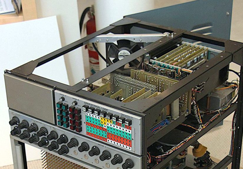
The famous 1969 restoration subject often discussed by vintage-computing enthusiasts is a Simulators Inc. Model 240 analog computer. It was described as a precision general-purpose desktop analog computer with room for up to 24 operational amplifiers, though one known restored unit contains 20. By today’s standards, that sounds tiny. By 1969 standards, it was an elegant laboratory tool: compact, reconfigurable, and powerful enough to solve serious engineering problems.

This machine came from a period when analog computers were still useful for fast scientific and engineering simulation. They were especially good at solving differential equations, the mathematical language of motion, feedback, vibration, heat flow, electrical circuits, and countless real-world systems. If a problem changed continuously over time, analog computing was often a natural fit.

The secret is that analog computers did not simulate time by slicing it into tiny digital increments. Their circuits evolved continuously. When properly configured, the output could appear almost immediately on a meter, oscilloscope, strip-chart recorder, or X-Y plotter. That made analog computers valuable for real-time simulation, especially before digital machines became fast, cheap, and convenient.

Patch Cables Were the Programming Language

Programming a 1969 analog computer did not involve typing commands into a terminal. There was no friendly blinking cursor. No compiler. No “unexpected token” error message waiting to ruin your afternoon. Instead, programming meant plugging cables into a patch panel.

The patch panel was the machine’s front-facing mathematical map. Each cable connected computing elements such as amplifiers, integrators, potentiometers, and multipliers. To build a program, the operator translated equations into circuit relationships. A wire might feed one voltage into an amplifier. Another might route an output into an integrator. A knob might set a coefficient. A relay might switch the computer between “initial condition,” “operate,” and “hold.”

This made analog programming extremely visual. You could literally see the structure of the problem. The downside, of course, was that the “source code” could look like a multicolored octopus wrestling a telephone switchboard. Debugging meant checking cables, voltages, scaling factors, and hardware behavior. A loose connection could be the analog equivalent of a missing semicolon, except with more mystery and possibly a smell of warm electronics.

Operational Amplifiers: The Heart of the Machine

The operational amplifier, or op-amp, was the central building block of electronic analog computing. Today, op-amps are common integrated circuits used in audio equipment, sensors, filters, instrumentation, and countless gadgets. In a 1969 analog computer, the op-amp was not just a supporting actor. It was the star.

An op-amp could add voltages, invert signals, scale values, and form the basis of integrators. When combined with precision resistors, an op-amp could perform summation and multiplication by constants. When combined with a precision capacitor, it could perform integration, one of the most important operations in calculus. That is why analog computers were so good at solving differential equations: integration was built directly into the hardware.

In the Model 240, a single op-amp was not merely a tiny chip doing all the work. Although integrated-circuit op-amps existed in the late 1960s, their precision was not good enough for demanding analog-computer use. Designers combined IC op-amps with additional circuitry, including chopper stabilization, to create high-performance amplifier boards. In other words, one “op-amp” in the computer could occupy an entire circuit board. Modern engineers may weep softly at the size, but they should also admire the craftsmanship.

The Chopper Stabilization Secret

One of the best secrets from this 1969 analog computer is its use of chopper-stabilized amplifiers. This technique helped solve a serious problem: drift.

Analog computers depend on accurate voltages. If an amplifier’s offset changes slowly over time, the mathematical result can wander away from the truth. That is bad news when the voltage represents something important, like velocity, pressure, or the state of a control system. A normal amplifier might work beautifully for audio, where tiny DC errors are not a disaster. But in analog computing, low-frequency and DC accuracy are essential.

A chopper circuit converts a slowly changing input into an AC signal, amplifies it more reliably, and then converts it back. This helps reduce offset and drift. It is a clever workaround that shows how analog engineers fought physics with more physics. The result was not simple, but it was effective. In the 1969 machine, the extra chopper-related circuitry helped turn ordinary electronic parts into precision computing elements.

Integrators: Calculus in a Metal Box

To appreciate an analog computer, you have to appreciate the integrator. In mathematics, integration can seem intimidating, especially if your memories of calculus involve caffeine, panic, and a textbook the size of a paving stone. In an analog computer, however, integration becomes a physical process.

An electronic integrator uses an op-amp and a capacitor. Current charges the capacitor over time, and the voltage across it represents the accumulated value. If the input represents acceleration, integration can produce velocity. Integrate velocity, and you get position. With the right circuit, the computer can model motion in real time.

That is why precision capacitors mattered so much. Leakage, tolerance, and stability directly affected the answer. The components inside a 1969 analog computer were not random parts from a bargain drawer. They were chosen because tiny errors could become visible mathematical mistakes. In analog computing, the hardware was the equation, so the quality of the hardware was the quality of the math.

Potentiometers: The Knobs That Held the Constants

Analog computers also relied on potentiometers to set parameters and scaling constants. A potentiometer is a variable resistor, but in this context it functioned like a carefully adjustable number. Many analog machines used multi-turn potentiometers so operators could set values accurately. A voltmeter could verify the setting before a run.

This gave analog computing a wonderfully tactile quality. Want to change damping in a mechanical model? Turn a knob. Want to adjust a coefficient in a control equation? Turn another knob. Want to make the result nonsensical? Turn the wrong knob and pretend you are exploring “alternative physics.”

The physical nature of the controls made analog computers useful in education and experimentation. Students could see cause and effect immediately. Engineers could vary parameters and watch a system respond. The experience was closer to operating a scientific instrument than using a modern laptop.

Analog Multiplication Was Surprisingly Hard

Adding and scaling voltages was relatively straightforward. Multiplication was more difficult. In digital computing, multiplication is routine because numbers are represented symbolically and processed through logic. In analog hardware, multiplying two continuously changing voltages requires a more elaborate circuit.

Some machines used parabolic or function-generator approaches. One mathematical trick is based on the identity that multiplying two values can be achieved through sums and squares. Squaring a single variable can be implemented with a shaped function circuit, while op-amps handle addition and subtraction. It sounds like taking the scenic route to the grocery store, but in hardware design, the scenic route is sometimes the only paved road.

The Model 240 included analog multiplier circuitry, and reverse-engineering such modules reveals just how much precision hardware went into functions that modern digital processors perform silently billions of times per second. Multiplication in analog form required careful design, precision resistors, temperature awareness, and patience. Lots of patience.

The Power Supply Was Not Boring

In ordinary electronics, the power supply is often treated as background infrastructure. In an analog computer, it is part of the foundation of truth. If the reference voltages are inaccurate, every computation can be affected.

The 1969 analog computer used precise reference voltages, including positive and negative 10-volt references, along with regulated supplies for the op-amps and other circuitry. Older tube-based analog machines often used much higher reference voltages, but solid-state designs allowed lower operating levels. Still, the need for stability remained critical.

During restoration work on this kind of machine, even a power-supply fault can become a detective story. Engineers must understand not only whether a voltage is missing, but how the regulator, reference network, amplifier cards, connectors, mechanical hardware, and thermal conditions interact. Vintage computing restoration is not just replacing parts. It is archaeology with a multimeter.

Hybrid Computing: When Analog Met Digital

By the late 1960s, analog and digital computing were not always enemies. In fact, some of the most interesting systems combined both. Analog computers were strong at continuous real-time simulation. Digital computers were strong at logic, storage, sequencing, and precise symbolic calculation. Hybrid systems tried to use each where it made the most sense.

Some analog computers included digital logic such as gates, flip-flops, counters, and switching controls. Larger hybrid systems connected analog machines to digital process computers through converters and control interfaces. Digital-to-analog converters could feed parameters into the analog side. Analog-to-digital converters could capture results. Logic interfaces allowed coordination between discrete and continuous domains.

This approach feels surprisingly modern. Today, many advanced systems combine digital control with analog sensing, signal conditioning, neuromorphic circuits, mixed-signal chips, and specialized accelerators. The 1969 analog computer reminds us that “analog versus digital” was never the whole story. The smarter question has always been: which kind of computation fits the problem?

Why Analog Computers Faded Away

If analog computers were so fast and elegant, why did they disappear from mainstream computing? The answer is not that they were useless. The answer is that digital computers improved at a breathtaking pace.

Analog computers were difficult to configure, maintain, scale, and document. Accuracy depended on component tolerances, calibration, temperature, drift, leakage, and noise. Reusing a program could require saving or rebuilding a patch panel. Complex problems required more hardware. Precision demanded expensive components. Operators needed deep technical understanding.

Digital computers, meanwhile, became faster, cheaper, smaller, and easier to program. Software could be stored, copied, edited, and shared. Accuracy could be improved by using more bits. Integrated circuits transformed digital performance. By the 1970s and 1980s, digital computing had taken over most roles once held by analog and hybrid machines.

Still, the disappearance of analog computers should not be mistaken for failure. They solved real problems in engineering, aerospace, education, industrial modeling, and scientific simulation. They were not primitive digital computers. They were a different species.

What Modern Engineers Can Learn From a 1969 Analog Computer

1. Hardware Can Teach the Math

A patch-panel analog computer makes equations visible. You can trace a signal from one module to another and understand how a mathematical relationship becomes a physical process. This is valuable for learning. Modern software can hide too much. Analog hardware makes abstraction tangible.

2. Parallelism Is Powerful

Analog computers operate naturally in parallel. Every part of the circuit participates at once. Modern computing is still chasing parallel performance through GPUs, AI accelerators, multicore processors, and specialized chips. The analog computer reminds us that parallelism is not new; it just used to come with more patch cables.

3. Precision Is a System Problem

In analog computing, accuracy depends on the whole system: resistors, capacitors, amplifiers, power supplies, thermal behavior, and calibration. That lesson still applies. Whether building sensors, robotics, medical devices, or scientific instruments, precision is never only about one component.

4. Interfaces Shape Thinking

Typing code encourages one way of thinking. Wiring a patch panel encourages another. Turning knobs and watching an oscilloscope creates immediate feedback. The interface changes how people understand the problem. That is a lesson for software design, education, and engineering tools.

The Human Side of Vintage Analog Computing

There is something charming about a 1969 analog computer because it feels both brilliant and stubborn. It belongs to a time when engineers could not simply import a library, open a cloud dashboard, or ask an AI assistant to explain why the build failed. They had to understand the machine down to the resistor network. They had to make mathematics behave inside metal, plastic, copper, and glass.

Restoring one of these computers today is a reminder that old technology is not automatically simple. In many ways, it is harder to understand than modern devices because there is less abstraction protecting you from reality. A modern laptop may contain billions of transistors, but most users never meet them. A 1969 analog computer introduces you personally to its components, and some of them seem to have opinions.

The machine also carries a quiet warning. Technology history is not a straight road from “bad old tools” to “perfect new tools.” It is a branching forest of ideas. Some paths become highways. Others become overgrown trails. Analog computing is one of those trails, and it may still lead somewhere useful.

Experience Section: Lessons From Exploring the Secrets of a 1969 Analog Computer

Spending time with the story of a 1969 analog computer feels like walking into an old engineering lab after everyone has gone home but the equipment is still warm. The first impression is visual. The patch panel grabs your attention immediately. It looks chaotic, but the chaos has rules. Every cable means something. Every connection is a sentence in the language of the machine. After years of thinking about computers as screens and keyboards, it is refreshing to see computation as something you can physically touch.

One experience that stands out is realizing how much responsibility the operator had. With a modern computer, we often blame the software, the operating system, the internet connection, or a mysterious “server issue.” With an analog computer, the user is much closer to the problem. Did you scale the voltage correctly? Did you set the initial condition? Did you connect the integrator output to the right input? Did the power supply stabilize? Did that precision component drift? The machine asks you to be careful, and it rewards careful thinking.

Another memorable lesson is that analog computing makes calculus feel less like a classroom punishment and more like a living process. Integration is not just a symbol on paper. It is a capacitor charging. Feedback is not just a block diagram. It is a cable carrying a signal back into a circuit. A differential equation is not trapped in a textbook. It becomes a behavior you can watch on an oscilloscope. For students, hobbyists, and engineers, that shift can be powerful. It turns abstract math into an experiment.

The restoration angle adds another layer of appreciation. When documentation is missing, the machine becomes a puzzle. Reverse-engineering a board means following traces, identifying components, measuring signals, comparing behavior, and making educated guesses. It is slow work, but it is also deeply satisfying. There is a detective-story quality to it. A failed voltage rail, a suspicious connector, or a drifting amplifier can become the clue that explains the whole system. The computer does not give up its secrets quickly; it makes you earn them.

There is also a surprisingly modern feeling in the analog-digital relationship. The old assumption that digital simply replaced analog now feels too simple. Today’s world depends on mixed-signal systems everywhere: phones, cars, medical sensors, audio gear, robotics, industrial controls, and AI hardware. Digital logic may dominate the headlines, but analog reality still sits at the front door. Sensors collect continuous signals. Power circuits manage real energy. Radios live in waveforms. The 1969 analog computer feels like a reminder that computation begins in the physical world.

The most personal takeaway is humility. A machine from 1969 may seem obsolete, but it embodies an astonishing amount of intelligence. Its designers understood mathematics, electronics, control systems, materials, tolerances, calibration, and human operation. They solved problems with the tools available, and they did it with elegance. Looking at the Model 240 and similar machines, it becomes obvious that “old” does not mean “crude.” Sometimes old means direct, disciplined, and beautifully honest.

If there is one experience-related secret worth carrying forward, it is this: analog computers teach patience. They make you slow down and understand the relationship between model and machine. They remind you that computation is not only about speed. It is about representation. A good computer, whether analog or digital, gives a problem a form that can be explored. In 1969, that form involved voltage, precision components, and a patch panel. Today, it may involve code, silicon, or cloud infrastructure. The goal is the same: turn a question into a system that can answer back.

Conclusion: The Future Hidden in an Old Patch Panel

Secrets From A 1969 Analog Computer is more than a nostalgic trip through vintage electronics. It is a window into a computing philosophy that valued physical modeling, continuous behavior, and real-time interaction. The Simulators Inc. Model 240 and machines like it show how engineers once solved complex problems with voltages, cables, amplifiers, capacitors, and carefully calibrated components.

Digital computers won the mainstream battle because they became flexible, accurate, affordable, and incredibly powerful. But analog computing never stopped being interesting. In fields such as neuromorphic design, mixed-signal hardware, scientific simulation, and energy-efficient computing, old analog ideas continue to echo. The 1969 analog computer may belong to history, but its secrets still feel alive.

And maybe that is the best part. Beneath the knobs and patch cables is a lesson for every generation of technologists: there is more than one way to compute. Sometimes the answer is not hidden in software. Sometimes it is humming quietly inside a circuit, waiting for someone curious enough to plug in the right cable.